When I was studying computer science at the University of Helsinki, I went to one machine learning course. During the first lesson, there was a prerequisites test, which I failed spectacularly, and gave up the course right there. After that, I did not look into neural networks for many years despite making my master’s thesis about optimisation algorithms in real-time strategy games, where they certainly could have been one viable solution.
Somewhat recently I was interested in stock trading. That inspired me to read a little about neural networks and I tried building one that predicts the stock market with Google’s open-source solution TensorFlow. Obviously, that did not work, but still, I learned the basics of TensorFlow, which is probably one of the best options to use if you want to get something real done. You only need to describe the network, give it a bunch of parameters and TensorFlow handles the actual implementation.
Some weeks ago I stumbled across these four great videos describing neural networks in a way that really increased my understanding of how they actually work. But still, I felt that the last piece was missing. To really understand what is happening and how I needed to implement one myself. All the way from scratch.
Recognising numbers – an approach with less math
For this project I chose probably the most standard schoolbook problem there is: recognising handwritten digits. This kind of image recognition task – while far from trivial – is one where artificial neural networks have been proven to work well countless times already. Also, large amounts of labeled training data is easily available.
If one wants to build an efficient neural network, the obvious and likely easiest way to go is to make heavy use of matrix operations and other linear algebra. I suppose that is one reason why python is a common language here, given its good library support for such things.
But that was not my goal. If I wanted to build a concrete understanding as possible of how the network works, I felt that for me personally, the math would be in the way, obscuring things, although I do see why many would disagree.
So instead I chose a more object-oriented approach to model the network, with a sprinkle of functional programming on top (don’t want to feel like a dinosaur after all, despite maybe having a minor 30’s crisis). My language of choice was Kotlin, which along with TypeScript is one of my clear favourites at the moment. I did not use any dependencies, everything is plain handwritten Kotlin.
Given that a random number generator would guess the digit correctly 10% of the time, I set my initial target to 15 % success rate, just to prove that the network is at least doing something right. As it turns out, this was rather pessimistic and to my surprise, the final success rate made it past 90%, and after adding some ad-hoc convolution layers it exceeded 96%. Let’s see how we got there!
What is it and how does it fly
First of all, I want to emphasise that this is not an area that I have extensively studied, so some of the terminology and theory here may be slightly inaccurate. But then again, the whole point of this post is to show that you can already get some pretty cool things done without spending a lot of time with your nose stuck in a book.
That out of the way, I will now first attempt to explain how an already-trained network functions. How does it get from a bunch of pixel values in the input image to a single number being the recognised digit?
Basic concepts
Most of this revolves around three very simple concepts, which are also at the center of my object-oriented model.
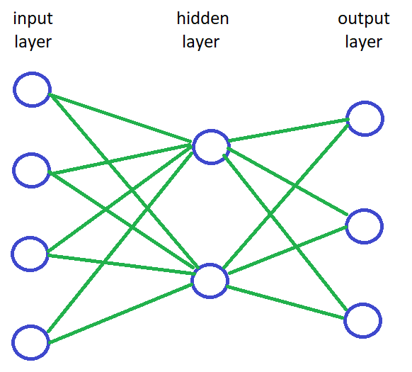
- A neuron, with a loose analogy to the brain, is a node in the network. Each neuron has an activation value; a number describing how active it is. You might also visualise the neuron as a light bulb and think of the activation as how brightly it is lit. Each neuron also has a value called bias, which could be thought of as a minimum power needed for the neuron to light up.
- Between neurons there are connections. Each connection has a weight, which describes the strength of the connection, i.e. how much the activation of the previous neuron affects the activation of the latter. Weight can also be negative, in which case when the input neuron gets brighter the output neuron gets dimmer and vice versa.
- While this may not really have an analogy with brains, usually the network is organised into layers. Each layer is simply a set of neurons. The very first layer is the input layer, the very last one is the output layer, and any layers between them are so-called hidden layers. In a most basic network, every neuron on every layer is connected to every neuron in the next layer. How many hidden layers there should be and how many neurons should each have is very difficult to know in advance. Mostly it is a matter of trial and error: keep trying different things until you get lucky and something gives good enough results.
Propagation from input to output
Now that we have laid out some terminology and described what the network consists of, let us next look into how it works and how it can be used.
First, we shall manually set the activation of each neuron on the input layer so that they somehow encode the input data. In this case, the input is a grayscale image of 28×28 pixels, each of them having a value of how bright/dark that pixel is. Our input layer will thus consist of 784 neurons, each of them associated with one pixel, and the activation value between 0.0 and 1.0 will be set to the brightness of that pixel.
Next, we will start moving on layer by layer. For every neuron, we will calculate its activation based on the connections from the previous layer. I will soon explain how exactly is each activation calculated.
Finally, we arrive at the output layer. In this classification problem where we are trying to recognise digits between 0 and 9, there are 10 different options. Thus our output layer should have 10 neurons. Once we have calculated an activation level for each of them, our best guess for the digit in the image is simply the index of the output neuron that has the highest activation.
Calculating activations
Calculating the activation of a neuron is done with a simple propagation function. At its core, it is just a weighted sum. You look at each neuron on the previous layer and multiply their activations with the weights of the associated connections. Then you just sum them up and finally add the bias of the neuron.
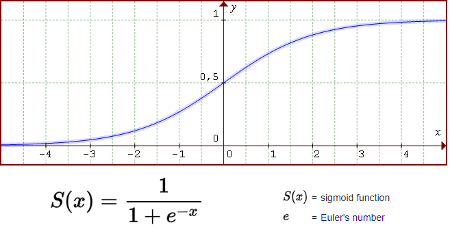
The last step we should do is to put the result through a so-called activation function. Here again, there are many alternatives that you can try, but the most classic option is a function called sigmoid. That function basically squishes the input from the previous step so that the end result is always between 0.0 and 1.0.
Class model and forward propagation implementation
Now we have a general understanding of the terminology. As mentioned, I chose to implement the network in an object-oriented model, so I know you must already be itching to see some UML diagrams. No worries, I got you, buddy!
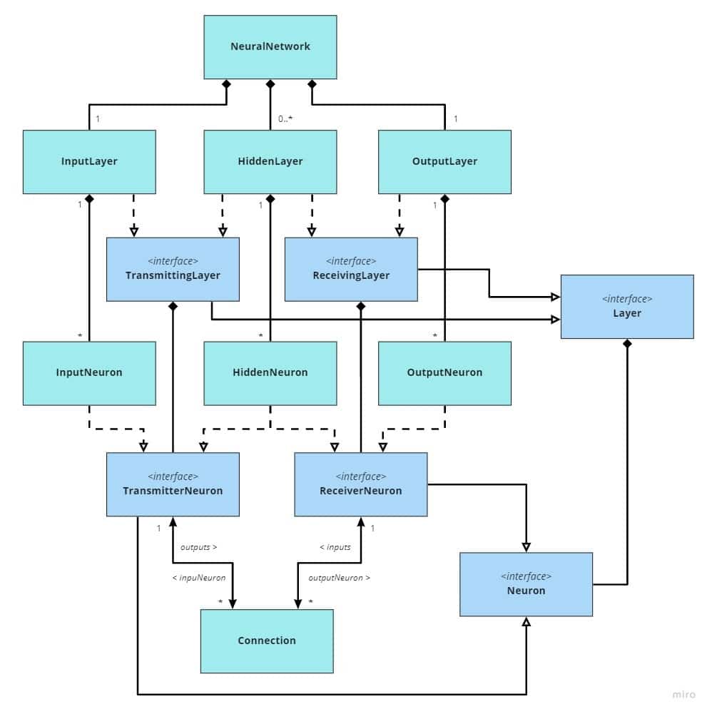
So essentially there are just those three concepts we talked about – neurons, layers and connections – but they have been broken down a bit more. For example, every Neuron has activation, but OutputNeurons on the OutputLayer have no further output connections since it is the last layer. Therefore, the outputs field is on the TransmitterNeuron interface, which is implemented by InputNeuron and HiddenNeuron but not OutputNeuron. Connection has weight and ReceiverNeuron has bias. That is pretty much all.
With these constructs, after we have set the activations on InputNeurons based on some image, the matter of propagating the activations forward all the way to the OutputLayer only requires calling one function for every ReceivingLayer in order

which in turn only calls a simple eval function for each ReceiverNeuron

As discussed earlier, the activation is calculated simply by taking a weighted sum of the input activations, adding the bias, and then crushing the result through an activation function such as sigmoid.
How to train your network
As seen above, implementing the network is very simple if you somehow already have a set of values for every single weight and bias. Assuming our network has those 784 input neurons, 10 output neurons and for example just one hidden layer of 16 neurons, that already means there are 784 * 16 + 16 * 10 = 12 704 connections with weights, and 16 + 10 = 26 biases (neurons on input layer do not have bias). A total of 12 730 parameters. Making the network ”recognise” something is all about finding values for these parameters that happen to cause certain inputs to produce correct outputs.
If we were to consider only one image, say one that represents digit 2, it would be rather easy to find some weights and biases even manually so that the output neuron associated with digit 2 would have activation close to 1.0 and every other output neuron would have activation close to 0.0. But that is of course not enough. We need to find values that simultaneously lead to correct answers with any of the thousands of training images representing different digits.
So how do we actually get those? The first idea might be to just randomly try different values until we find something that works. Unfortunately, since there are so many parameters, that would be way too slow. It would be like trying to navigate in a huge forest without a map or a compass while blindfolded. Fortunately we can devise sort of a compass by using a process called gradient descent.
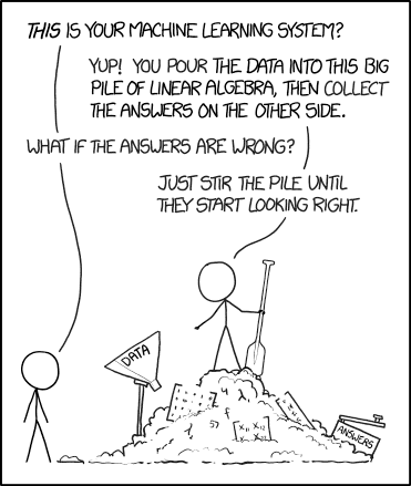
Credit: https://xkcd.com/1838/
Gradient descent and backward propagation
If you really don’t like math, skip this chapter. ;)
First, we need to define a cost function, which tells us how badly the network behaves at the moment. The cost function typically used in neural networks is
C = (a – y)2,
where a is the activation value of an output neuron and y is the value we would have wanted it to be. That of course needs to be summed up overall output neurons and also averaged over sufficiently many training images. Now we have a single number to measure how bad the network is and we can improve the network by trying to minimise that.
Now imagine that you are standing on a hillside. If we think of the cost function as how high you are, that means you want to go down the hill and find the bottom of the valley. However, it is night and you can not see anything. In that case, you could try to feel the ground around yourself, find out the direction where the descent is steepest, take a step towards that direction and repeat. By using this algorithm you are at least guaranteed to soon end up at the bottom of some valley. That is the idea of gradient descent.
So we could just adjust the parameters a tiny bit and see which way the cost function decreases the most. Unfortunately, the number of parameters is still an issue. Basically, we are not standing on a normal hillside, but on one that is 12 730 dimensional, so there are just too many possible directions to feel around. So again we need to reach into the toolbox of mathematics to find something that helps us speed up the process.
While the cost function seems to be a function of the activation values, those, in turn, are functions of the network parameters. Therefore, the cost function is in the end just a function of all those different parameters, albeit rather complex ones, and it is possible to analytically find a partial derivative of the cost function with respect to each different parameter. Then in order to take a step towards the right direction, we simply evaluate the partial derivative for every parameter, multiply it with some small constant (a step size) and subtract it from the parameter’s current value. Now we have a working compass that tells us the direction to go!
I will not go too deep into the mathematics of how to derive those partial derivatives, but if you start from the last layers, it starts off quite simple. For example, with some high school mathematics, you can see that if
C = (a – y)2 = a2 – 2ay + y2
then the partial derivative of it in respect to a is:
dC/da = 2a – 2y = 2(a – y)
Next, we need to consider how for instance some weight w0 would affect a. That is, what is the partial derivative da/dw0. Once we have that we can use the chain rule to find the partial derivative of the cost function C with respect to the weight w0
dC/dw0 = da/dw0 dC/da
As I promised not to dive too deep into mathematics, I will not even try to show what is that da/dw0, but hopefully, you now have at least a very vague idea of how we would approach solving these derivatives. As you might have guessed, the derivatives get rather complex once you move further away from the output layer, since there are so many things that chain together. Fortunately, though, it turns out that once we have figured out all the partial derivatives of the last hidden layer LN-1, it is enough to find partial derivatives of the activations on that layer with respect to the parameters of the second last layer LN-2. Then we can chain those together to find the partial derivatives of the cost function with respect to the parameters on layer LN-2. This way we only have a limited amount of math to figure out, and then we just apply it recursively, moving back one layer at a time. This is called backward propagation.
Implementation of the training algorithm
It is quite possible that I derived some of the equations incorrectly, but be as it may, the end results are decent and with machine learning that is all that really matters, so I will dare to present my code that relies on those equations. If we take those for granted, my solution becomes quite simple.
First, we need to do a couple of small additions to our data model. To be able to average partial derivatives for weights and biases over multiple images and to keep track of partial derivatives by neuron activations when back-propagating we add these lists:
- Connection
derivativesOfCostByWeightPerSample: List<Double>
- ReceiverNeuron (i.e. HiddenNeuron and OutputNeuron)
derivativesOfCostByBiasPerSample: List<Double>
- HiddenNeuron
derivativesOfCostByActivation: List<Double>
For OutputNeuron we also add a field desiredActivation: Double which will contain the expected activation value based on current image.
Then the training algorithm consists of these 8 relatively simple steps:
Step 1
Clear derivativesOfCostByBiasPerSample for every neuron and derivativesOfCostByWeightPerSample for every connection
Step 2
Clear derivativesOfCostByActivation for every HiddenNeuron
Step 3
Use a training image as input and propagate forward to set all activation values. Set desiredActivation for each OutputNeuron to 0.0 or 1.0 based on what digit the image represents.
Step 4
Call the train function on each OutputNeuron:
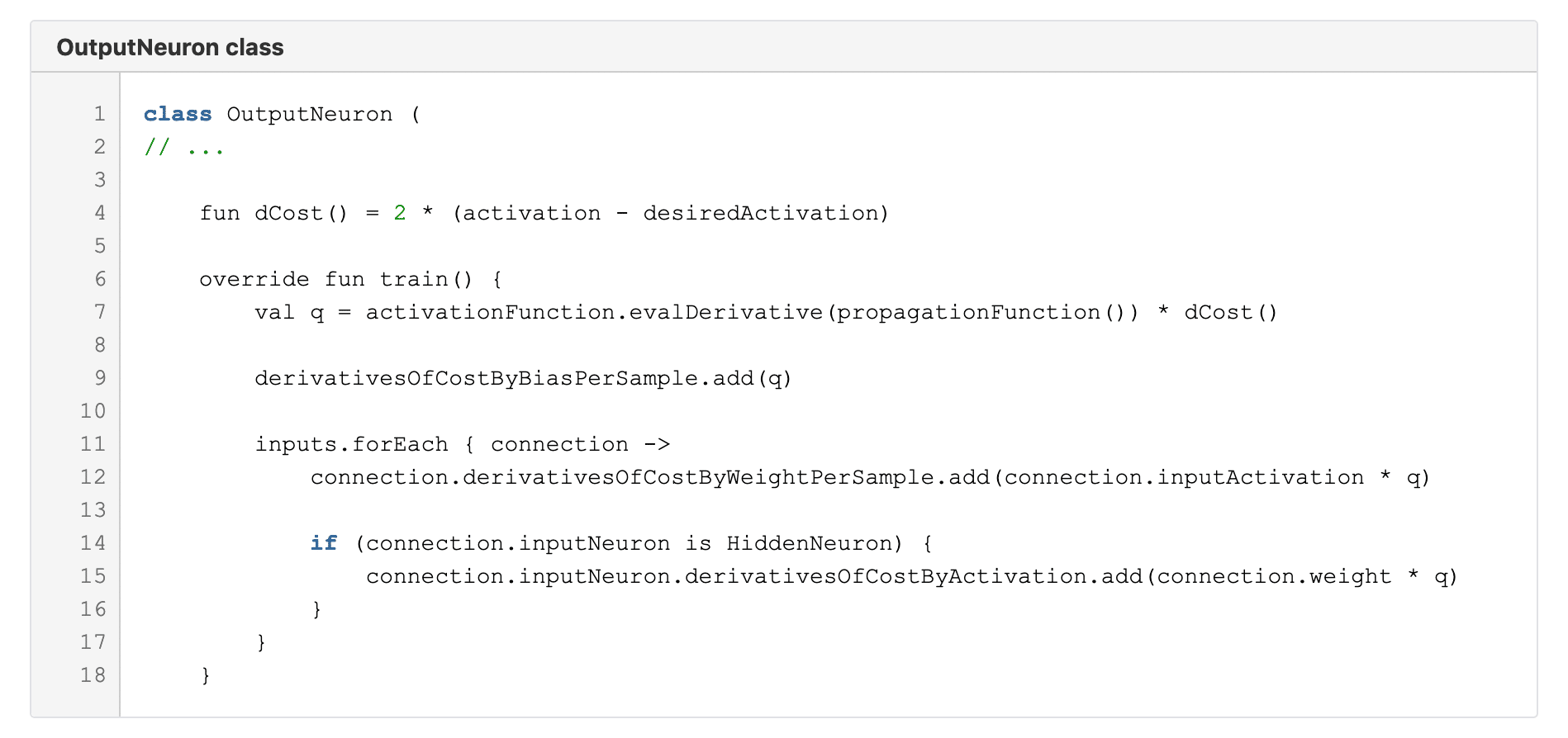
Here on line 4 we have the previously discussed derivative of the cost function. The train function starting on line 6 simply calculates some values and adds them to lists.
On line 7 we need the derivative of the activation function, which in the case of sigmoid is

Step 5
Call the train function on each hidden neuron on the last hidden layer. Then do the same for every neuron on the previous layer, and so on.
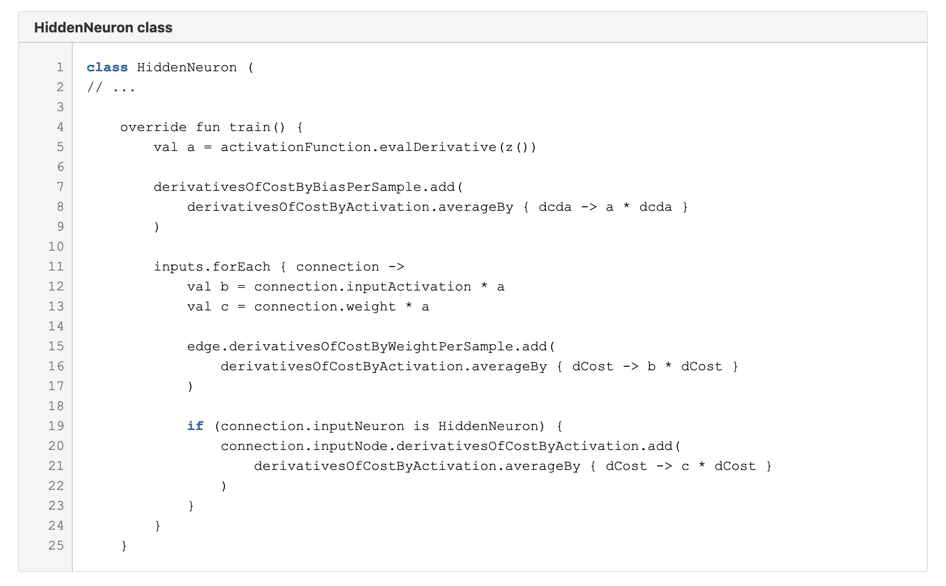
Here we again just calculate similar stuff and add the results into lists. On lines 8, 16 and 21 you get a taste of Kotlin’s nice functional API with the averageBy function. The lambda you give it is evaluated for each element of the list and then an average is calculated from those. Clean, concise and simple!
Step 6
Repeat steps 2-5 for at least some portion of the training images.
Step 7
Call the nudgeParameters function for each ReceiverNeuron, which will adjust all the parameters based on the previously calculated results.

Here on line 5 I chose to limit the bias always between -0.8 and 0.8.
Step 8
Repeat the steps 1-7 until the results no longer improve. That is all!
Online demo
For presentation purposes, I also wrote this demo application with React and Typescript. There you can draw a number yourself and the app will try to recognise it. The results are not quite as great as with the pre-made test data set, possibly due to differences in normalising the images, but still rather impressive in my opinion. How it works is that I implemented the forward propagation part of the network also in TypeScript and imported a pre-trained network from a JSON file that I had exported from the Kotlin version. The rest is just basic React and HTML5 stuff.
Feel the force, read the source
I challenge you to go through the same exercise yourself during some rainy weekend to make use of these times of isolation. I feel this was a very interesting and rewarding little project. However, you may also have a look at all the code in my full solution and use it as you wish: https://github.com/Joosakur/neural-network-test
Are you eager to learn something new? Are you interested in challenging tech projects? Check out also Join the Crew


